
Bet sequences, an analysis
Level ∞ - BILL BETTOR

Do you have a friend who likes betting and would like to sharpen his/her action? Help them on their path by sharing the BowTiedBettor Substack. Win and help win!
Welcome Degen Gambler!
Suppose that you’ve managed to develop a promising betting model. The basic backtests have been looking good and by now you believe the time has come to test it live. You’d however prefer to have gained some insight regarding the sequence of bets that you and your model are about to generate prior to launching it. Questions such as the following arise:
What’s there to “expect” from the bet sequence/process? Which paths are possible, which are plausible?
What’s the probability of losing money over, say, 420 bets despite having an average EV of, say, 10 %?
What’s the necessary amount of settled bets to reach any kind of conclusion regarding the efficiency of the model?
Note: Efficiency of a betting model = does it make money or not? Everyone can hit +80 % during a NHL season [bet all the < 1.20 and you should be good], this number alone tells you absolutely nothing. Probabilities don’t put food on the table, payoffs do.
Today, we will make an effort to provide solutions to such inquiries. We will conduct a comprehensive examination, utilizing both classical probability theory and modern simulation techniques, of the cumulative P&L (profit and loss) and ROI (return on investment) - two random sequences/processes created by placing numerous bets within a certain time frame.

A mathematical perspective
When faced with a theoretical problem, one of the most powerful approaches is to break the problem into small pieces, gain insight about those, then reconstruct and give the initial problem a second try, now equipped with the newly attained knowledge and a greater understanding of the matter.
A betting sequence/process is, as the name suggests, a sequence of bets, with bets arriving one at a time. Therefore, by way of the above approach, we begin by breaking the analysis of the full sequence into a smaller subproblem, in this case an examination of a single bet, or perhaps more relevant for our ambitions, the P&L of a single bet.

Note: One could throw away either one of odds, expected value or probability from the above definition without any loss of information (why?). For clarity we’ve nevertheless chosen to include all of them.
What’s a random variable, one might ask? Easy! A measurable function from a probability measure space to a measurable space. WTF? Yep, just kidding.
For our purposes a random variable is a variable that can take a finite amount of values, each with a certain probability and such that the probabilities add up to one.
Example: X, a variable that holds information about the result of a flip of a coin, is known to always evaluate to either 0 or 1. With probability 0.5 [heads] it’s 0 and with the remaining 0.5 [tails] it’s 1. Thus, X is a *random* variable since it depends on the outcome of the coin flip [a *random* experiment].
To proceed in a similar fashion as in the example above, we’d like to come up with a precise “random variable-definition” of the P&L of a bet. Since we want it to possess complete information regarding the result of the bet, we’ll let it take two possible values.
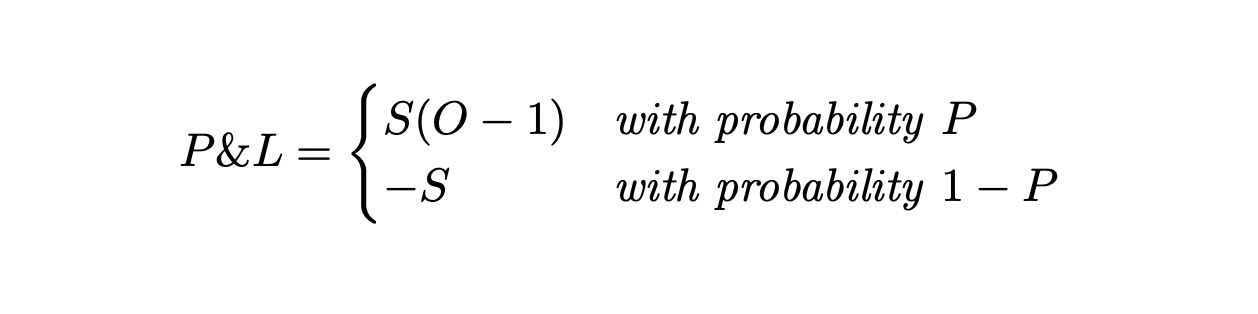
Recall that S = stake and O = odds. In other words the P&L random variable keeps, as the name suggests, track of the net profit/loss obtained from the bet. If the bet wins, it evaluates to the net profit [stake x net odds = net profit]. On the other hand, if the bet loses, the full stake is lost and so the P&L becomes negative the stake [-stake = net loss].
Indeed, this definition seems reasonable.
Having solved this subproblem, we now return to the original mission. To analyze the full cumulative P&L process we’ll have to take all the n bets into account, not only one of them. But this is easy, right? We simply repeat the above procedure for each and every bet in our sequence. Then, when this has been done, we sum them all up to generate the cumulative P&L.

Furthermore, let’s do a slight adjustment and see if anything of interest may appear: we divide the cumulative P&L by the total turnover [sum of all stakes] during the period,

Interesting!
At this point we’ve managed to construct formal random models [random since they both depend on the outcomes of the games the bettor is placing bets on] for two crucial betting processes, the cumulative P&L and the ROI. Thus we are in a good position to further deepen our exploration of them and analyze their different properties:
Distributional properties. Perhaps we’re interested in the full probability distribution of the ROI after the first 200 bets. Is this possible to obtain?
Convergence properties. Do the measures converge, and if so, how fast? As mentioned in Betting 101, we somehow ‘feel’ that the ROI should converge to the true, underlying EV as the number of bets increases. Meanwhile, it seems unlikely that the cumulative P&L will converge to anything. If we’re betting +EV games it’ll drift upwards, else it’ll drift downwards, right?
Autist challenge: can you come up with examples where the cumulative P&L in fact does converge?
Cumulative P&L
As already mentioned we don’t expect interesting things concerning convergence to pop up here.
What about its distributional properties?
In general, with zero restrictions/constraints on the behaviour of the individual bets we cannot say much. Well, we may note some trivialities,
Being a sum of a collection of discrete random variables, the cumulative P&L must itself be discrete.
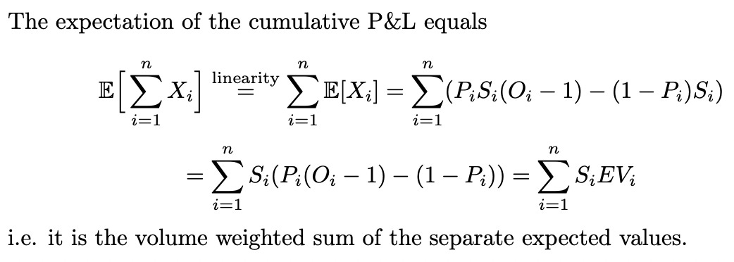
Expectations behave like “expected”.

Assuming independence between bets we discover that the variance increases with increasing n. This agrees with our intuition and is a consequence of the fact that the cumulative P&L is an unnormalized measure.
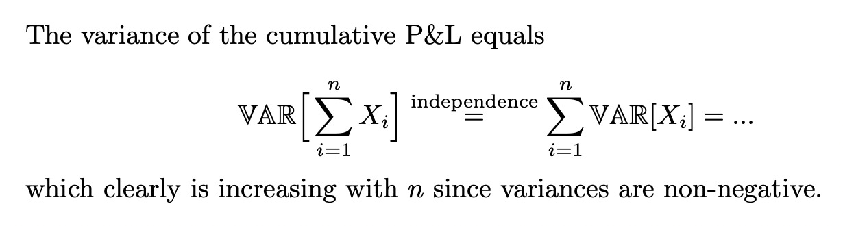
Note: The assumption of independence between bets could be invalid for many reasons. An example: several bets in one horse race. Another: a degen gambler increasing size with drawdowns to ‘win it all back’.

but to obtain general information regarding the resulting probability distribution we’ll have to resort to Monte Carlo methods.
Monte Carlo methods are a class of computational techniques that use random sampling to estimate numerical solutions to problems that may be difficult or impossible to solve using ‘standard’ methods. With zero structure [as in this case with varying stakes, odds & probabilities], the generation process of the cumulative P&L becomes an excellent example of such a problem.
ROI
In our Betting 101, the following was stated,
There is an interesting connection between the expected value and the ROI measure. If one views the expected value as an abstract concept handling “true” probabilities, the ROI measure is its practical counterpart, only taking a finite, often small, sample into consideration. However, as the number of bets increases one may expect the ROI to converge to the true EV of the betting sequence, making them both more or less equivalent. A more detailed discussion on this is coming!
Expecting & believing something is one thing. Actually proving it is another. Moreover, during the course of testing a hypothesis, it is common to uncover significant flaws in your current understanding and gain valuable insights that had not been previously considered.
Therefore, let’s try to prove our hypothesis: that the ROI does in fact converge to the true EV as the number of bets grows large.
ROI - Trial #1 [zero assumptions, full generality]:
Recall the ROI measure:

To prove that a random variable [in this case the ROI measure] converges to a given real number, one has to show that by picking a large enough number of bets, one is “guaranteed” to come “arbitrarily” close to the given value.
Autist note: Unfortunately the notion of probabilistic convergence is far from straightforward, making it difficult for us to be 100 % precise here. There are four different kinds of convergence [conv. in distribution, conv. in probability, conv. almost everywhere, conv. in p’th mean], all suitable for different occasions. To simplify matters we’ll restrict ourselves to convergence in probability which translates into the following: you give me *any* probability [say 0.05] as well as *any* small number [say 0.005]. Then, if I’m able to provide you with a large enough number of bets [say 12 000] such that the true probability of the ROI being outside the “small number-distance” [0.005 here] of the EV is *at most* the provided probability [in this case 0.05], the ROI is said to converge in probability to the EV.
With zero assumptions, the statement ‘the ROI converges to the EV’ will however be a very, very difficult proposition to prove. Why? Because it’s simply not true. Without restrictions on the stakes, probabilities and odds, there are a myriad of counterexamples that make any kind of convergence impossible.
Example of a counterexample: A bettor has taken the notion of ‘bet more’ literally and triples his average bet size at every 100’th bet. Thus, his ROI will at all times be heavily dependent on the ~ last 100 bets no matter how far into the future we go, ascertaining that the ROI measure will keep jumping around and refuse to ‘stick’ anywhere.


We conclude that we in fact *have to* introduce constraints if we hope to find any interesting properties.
Note: The code for all examples & simulations throughout this discussion lives here.
ROI - Trial #2 [perfect assumptions, independent, equivalent bets]:
If we instead look at the other extreme, where we assume independence and equivalence of all bets throughout the betting process, we hope to see neat convergence results. If not, well, then we won’t see convergence anywhere, right?
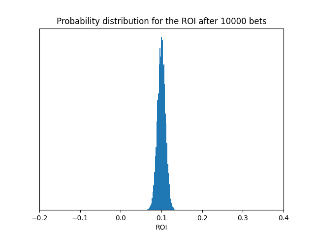
Example: A bettor is betting $1 on 2.00 outcomes, each with a probability of 0.55, over and over again.
Since the EV in the above example is 10 %, we expect the ROI to converge to this value [0.10].
In probability theory, one of many laws of large numbers states the following:
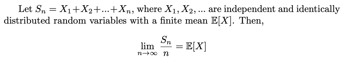
In our case we may identify the S_n variable in the theorem above as the cumulative P&L, and S_n/n the ROI after n bets. Since E[X] equals 0.10, with X being any one of the independent & identical bets of $1 on 2.00 outcomes [having 0.10 EV], the theorem guarantees that the ROI does indeed converge to the expected value. Great news!
The next question: how fast is the convergence? To gain some intuition on this, we’ll look at a couple of simulations prior to delving deep into the theory.

Cool, you think, after glancing at the graph for half a second. INSPECT IT FOR A WHILE, THINK HARD & LEARN INSTEAD! As you can see, it takes time, probably far more than you’d guess, to reach (or at least approximate) ‘truth’.
“Perfect world“ [independent, identical bets] ROI, theory
It’s time to continue our analysis of the ROI and its speed of convergence by going full math ‘tism, i.e. we’ll now examine the question from a purely theoretical viewpoint. To begin with, we’ll have a look at the ROI’s distributional properties. In fact, once the complete probability distribution of the process is derived, determining the process's position at various points in time becomes straightforward. This, in turn, makes it relatively easy to determine characteristics such as the rate of convergence.


Finally, we conclude this section with plots of the probability distributions [pictures tell more than thousands of equations] of the ROI for different N. Code as before on Github [LINK].


Welcome to Monte Carlo!
Now that we’ve analyzed the two edge cases, zero constraints and a maximum amount of constraints, we’d like to see what share of the assumptions we can drop while still retaining the nice convergence properties [since all bettors love to shout about the law of large numbers, it would be sad if it didn’t even apply to their betting, wouldn’t it?].
A non-triviality arises quite quickly though. As we begin dropping off assumptions, the theoretical parts, which by the way are on a quite sophisticated level already, will soon become more or less impossible to handle. Consequently Monte Carlo simulations will be the only reasonable way forward and therefore we’ll at this moment make a full transition into analyzing bet sequences purely on the basis of simulation techniques.
Autist note: If you’ve come this far & actually want to understand [using maths, not code] the precise assumptions one may drop without removing ROI → EV, we’re happy to discuss this further either in DM’s or in our Discord server.
Playing around with and meditating on simplified Monte Carlo simulations, or "alternative histories", is the best way to figure things out.Simulating alternative realities
To make matters more interesting, we’ll have a look at a real data set containing actual betting data.
Somewhere in the world there’s a bettor applying a specific horse racing model on a daily basis. Earlier this week he placed his 500’th bet for the year with this model and after pondering the result for a while he’s curious to learn how much of an outlier the latest 500 bets have been. From earlier investigations he’s almost certain that the true EV for the model is ~ 0.15. Furthermore, he’s also interested in discovering the likelihood of the ROI conditional on an EV of -0.15, the default margin applied by the bookmakers in the markets he’s operating in.
He’s been kind enough to provide us with an Excel file containing the data for the 500 bets.
Okay, let’s help the bettor!
We’ll run two experiments. In the first case we’ll assume that the EV is constant at 0.15/bet, in case 2 the assumption will be an EV of -0.15/bet. By using the odds [from the data file], the probability of a given bet winning is easily calculated as:
For each case we’ll then run 10 000 simulations for the cumulative P&L and 10 000 simulations for the ROI to learn a bit about which paths are possible and which are plausible.
Note I: For simplicity we’ll restrict today’s analysis to a sequence of 500 bets, i.e. the exact length of the historical data file. If one would like to investigate the matter on a longer time-frame [e.g. 1 000 or 10 000 bets] and/or begin with a smaller data set, we’d recommend using bootstrapping techniques to generate a sequence of wanted length.
Bootstrapping is a statistical method that involves resampling from the original dataset to create new samples that are used to estimate statistical properties of the population. The idea is to simulate the process of randomly drawing new samples from the same population to better understand the uncertainty associated with our estimates. Bootstrapping is useful because it allows us to simulate random processes and estimate the variability of our estimates without having to make assumptions about the underlying distribution of the population.
Note II: The assumption of a constant EV throughout a bet sequence is *always* invalid in practice, and even more so in cases where the gambler doesn’t operate within a certain odds range [as in our case, take a look at the data]. To illustrate why, suppose there’s a 1.04 bet included in the data. Then this bet automatically disqualifies all the other ones from an EV of above 4 %, which of course is nothing but stupid. However, to incorporate this into what we’re doing we’d have to include both randomness as well as an odds-dependence in the modelling of the EV, a procedure that is better left for the real turbos to perform on their own.
We proceed by creating two new columns with the assumed probabilities for each game. Next we load the updated dataset into Python. After that we’ll simply run the 10 000 simulations and see what happens. Additionally, the total stakes [which is a necessary metric to calculate the ROI] during the bet sequence was $112 768, a number we’ll simply hard-code into the Python program.

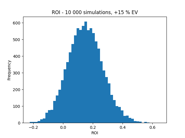
Case 1: +15 % EV
Results of the simulations below. Note that the actual ROI for our bettor was ~ 33 %. According to the simulations and assuming a 15 % EV, obtaining either this or an even higher ROI has a probability of ~ 7 %. Moreover, it should be observed that the probability of losing money over this 500 bet sequence, despite the +15 % edge, is about 10 %.
Statistical note: You may recognize this 7 % value from the statistical literature as the p-value [if you’re a p-value guy → definitely NGMI, 100 % a measure made for ‘tards] for the test of “EV is 15 % or less”.

Case 2: -15 % EV [default margin, i.e. betting randomly]
Again results below. This time the probability of obtaining at least such a ROI [33 %] has dropped severely to ~ 1/1000 [good news for our friend!], while the probability of losing money has increased to ~ 92 %.


Inverting the process & learning the truth the Bayesian way
Up until this point we’ve, perhaps without you even noticing, restricted our analysis to a certain perspective. Throughout the exploration we’ve *conditioned* on a specified EV and, *given* this EV, investigated possible real-world realizations. Indeed, if you’re fairly certain about your EV, this is an informative way of learning what the future may have in store for you. However, this is rarely the case in reality, right? In the real world no one really knows their true EV. Therefore, a more realistic and hence more interesting question is the converse: *given* a certain P&L, what conclusions can you draw about your EV?
Having read both our introduction to conditional probability & Bayes Theorem as well as part 1 in the Bayesian thinking & inference-series, the inverted thinking in the above paragraph should remind you of something. Indeed, Bayes!
So far, we’ve been working with the following probability,
however in practice we’re primarily concerned with the converse,
since after observing a ROI for our real world betting, we’d like to learn about the underlying EV to conclude whether our model is any good or not.
Using Bayes Theorem, we have,
with P(EV) the prior probability of the EV [which incorporates our initial beliefs of the quality of the model/bettor] and EV_range the range of possible values the EV might take. In plain english, what we’re doing is the following,
Initially, we construct a model where we claim that the EV might take on a certain range of values [for example everything between -0.5 to 0.5]. For every such value, we compute the conditional probability of observing the real-world sequence of bets [as in earlier sections]. If this probability is *high*, then the data indicates a certain plausibility of this EV. On the contrary, if the real world bet sequence is extremely unlikely to have been observed for the said EV, then, by actually observing it, we must of course respect the newly discovered information and deem that hypothesis less likely than before.
Example: You’re on a vacation in Brazil & there’s this guy offering everyone an odds of 2.50 on heads on the next coin flip. Since you’ve been brainwashed into thinking a coin flip is 50/50, that’s your initial belief. However, after observing 2 heads and 8 tails over the next 10 flips, you begin to seriously question whether the coin is loaded or not - you’re assigning larger and larger probabilities to heads as long as the data keeps pointing in that direction.
The beauty of Bayes is that it provides a perfect recipe for the conversion of this intuitive thinking into formulas!
To illustrate the method, we’ll in fact do exactly as in the above description and assume the EV to, with probability one, be in the interval [-0.5, 0.5]. Furthermore, to simplify things we’ll assume a uniform prior over this interval [i.e. our initial belief is that any EV between -50 % and +50 % is just as likely]. Then, we’ll *learn from the data* and update the probability of different EV’s accordingly. As more data arrive we continually adjust our distributions and beliefs.
Note: You’ll never agree with anyone on the choice of prior, but who the f*ck cares. We’re not here to write papers and engage in pointless discussions, but instead to learn betting & make money off that knowledge. If your priors are bad you’ll lose money. If they are good you’ll make money. Easy as that. If you’re investigating a newly launched bet picking service and you believe the founder of it to be extremely talented, of course you’ll want to incorporate that belief into your prior model and probably invest in him at an early stage. On the other hand, if you deem him stupid, you’ll give the negative EV’s greater weight & require him to perform on point for much longer until you’re convinced he knows what he’s doing. Makes sense, doesn’t it?
Output from the Bayesian analysis of the historical bets made by the horse racing bettor below. Inspect our code if you’re curious about the computational aspects [highly recommended, you’ll learn a lot by thinking about the logic of a Bayesian inference tool, in this case a very basic one].


Learning from data is sloooooooow… probably much slower than you’d think before seeing those graphs.
*Note that all the results rely on the constant prior assumption.
Conclusion
If you’ve made it this far you’re a certified autist so congratulations on that!
Concluding remark: what was to be said, has been said. We hope you’ve picked up a decent chunk of knowledge on the development of a bet sequence through time, and wish you best luck with *yours*!
Stay toon’d for more interesting betting material.
Until next time…

Disclaimer: None of this is to be deemed legal or financial advice of any kind. These are *opinions* written by an anonymous group of mathematicians who moved into betting.
Apologies if dumb question but in the last section (obtaining EV with real P&L), how do we take into account (in the code) a situation where the bet was a push? I tried a modification but that 2x'd the EV if all other parameters remain the same (N bets, real ROI).